Embedded Linux / Buildroot

I undertook this learning project to understand how software on a Raspberry Pi connects to the Linux system and hardware beneath it. Rather than stopping at running an application, I worked through the tools used to build target software, the components needed to deploy a Linux environment, and the interfaces through which programs reach the kernel and physical devices.

The application work brought those layers into focus. I implemented an OpenCV plate-processing pipeline, added brightness and contrast preprocessing informed by my photography experience, and produced annotated pedestrian-detection outputs. Alongside that work, I configured Buildroot, integrated a small system call, exercised kernel modules and character-device operations, and programmed GPIO-based outputs.

Technical scope: Raspberry Pi 3-family hardware; Linux host and virtual-machine environments; ARM GNU tools; QEMU and GDB; Buildroot; Linux kernel interfaces; C and libgpiod; Python, OpenCV, NumPy, and imutils; introductory TVM and RPC experiments.

Together, the work traces a practical learning journey: from preparing software for another architecture to observing kernel behavior, controlling peripherals, and examining application outputs. I documented the procedures and results so that I could connect what I configured with what actually happened on the target.

License Plate Recognition

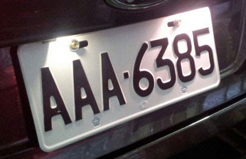
The plate-recognition work brought several image-processing concepts together in one application. I wanted to understand how a photograph becomes a sequence of recognized characters, and where that sequence can go wrong. I implemented and examined a pipeline that locates a plate, corrects its perspective, separates its characters, and compares them with templates.

I worked from an existing contour-and-template example using Python, OpenCV, and NumPy. My work involved carrying out the processing flow, inspecting its outputs, and extending it with histogram-based illumination adjustment, coordinate annotations, and basic execution-time observations. The underlying OpenCV operations and reference pipeline were existing building blocks; the learning came from connecting them, examining their assumptions, and making targeted modifications.

From a photograph to a plate region

The input was a saved vehicle photograph loaded from a file, with a separate directory of character templates. This kept the experiment focused on processing a known image rather than introducing a live camera-capture stage. I retained the original color image for the final overlay and converted a processing copy to grayscale, giving the subsequent stages a single intensity channel to work with.

After the illumination adjustment described below, I applied bilateral filtering. Its purpose was to reduce local intensity variation while retaining useful boundaries before edge detection. Canny then converted intensity transitions into an edge map. This gave contour analysis a representation of potential boundaries rather than asking it to work directly with the full photograph.

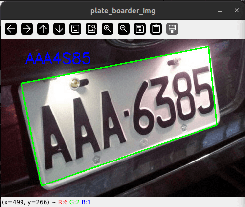
The localization step sorted contours by area and examined the ten largest. Each was approximated as a polygon, and the first candidate with four vertices was selected as the plate boundary. This is a straightforward geometric heuristic, not a trained plate detector: a rectangular object elsewhere in the scene can satisfy the same rule. The saved implementation also raises an error when it finds no four-point candidate, rather than recovering through another localization method.

I used the selected corners to define a perspective transform into a 320 × 150 plate region. This reduces the geometric variation passed to segmentation: characters photographed at an angle are brought into a more consistent rectangular frame. The transform depends on the chosen boundary and corner ordering; it cannot compensate for choosing the wrong object or reconstructing a hidden edge.

From the plate region to characters

The rectified grayscale plate was converted to a binary image using Otsu thresholding, then inverted so that character regions could be treated as foreground. The threshold is selected from the image's intensity distribution rather than set to one fixed value for every input. This prepares the image for connected-component analysis, but separating foreground and background still depends on the image content.

I then applied one erosion followed by one dilation using a 3 × 3 kernel. This opening operation is intended to remove small foreground noise before segmentation. It also introduces a tradeoff: thin strokes or small details can be altered along with unwanted pixels. The choice matters because the next stage treats connected regions as candidate characters.

The component-selection routine used region areas to choose seven candidates after skipping the largest region, which the implementation assumes is background. I ordered the extracted regions by their horizontal positions so that matching results would form a left-to-right string. These assumptions keep the example compact but make it specific to a seven-character layout. Noise, touching characters, or a broken stroke can change the component count or area ranking; the routine does not establish that every selected component is actually a character.

Each extracted region was resized to 18 × 36 pixels to match the template scale. For each region, the program compared all available templates with normalized-correlation matching and selected the highest-scoring candidate. This makes the matching process inspectable, including a score for each selected character, but the best available match is not necessarily correct. The routine does not reject a character simply because its best match is poor, and differences in font, stroke shape, or segmentation can carry through to the final string.

Engineering challenge: illumination and contrast

While examining the pipeline's limitations, I focused on poor lighting and reflection. Both can affect the intensity boundaries used to locate the plate and separate its characters. Rather than changing the matching stage first, I drew on my photography and image-editing experience: when a picture is dark or lacks tonal separation, I look at its brightness distribution before deciding what adjustment to make.

I implemented an automatic brightness and contrast function immediately after grayscale conversion. It builds a 256-bin histogram and its cumulative distribution, then uses a clipping percentage to find lower and upper intensity bounds. With the recorded default of 1%, the clipping allowance is divided between the two ends of the distribution. The function calculates a linear scale and offset to stretch the selected range across 0–255 and applies that mapping before filtering and edge detection.

This was a targeted preprocessing modification to the existing pipeline. The purpose was to give later stages a more useful intensity range without letting a small number of extreme pixels determine the adjustment. The report preserves the function, its insertion point, and before-and-after image treatment; the saved source also contains the function and its call.

The result supports that the adjustment was implemented and examined, not that it increased recognition accuracy. There is no controlled image set comparing recognition with and without it. A global intensity stretch also cannot recover obscured detail or solve every local reflection. For a follow-up, I would compare both versions on the same varied inputs and record localization, segmentation, and character errors separately. That would help identify where the adjustment helps and where a different approach is needed.

Results and what I learned

I used visual outputs to connect the final string to the decisions made earlier in the pipeline. The recorded results include a processed plate, character-region displays, a boundary overlay with corner coordinates, and terminal matching candidates. This made it possible to inspect whether an unexpected character followed from selecting the wrong region, segmenting a poor character shape, or choosing an unsuitable template. These are points to investigate, rather than documented diagnoses for every error in the sample.

Some predicted characters visibly differ from the photographed plate. The result demonstrates an implemented end-to-end processing flow, with a useful record of intermediate behavior, rather than a general-purpose recognition system. I also recorded execution time before output-image generation and inspected deployment storage, but did not establish comparative performance measurements. A separate OpenALPR installation and command-line experiment remains distinct from this Python implementation.

The main lesson was how strongly the stages depend on one another. Template matching cannot repair an incorrectly localized plate, and a clearer image does not guarantee correct segmentation. Working through the intermediate representations helped me reason about those dependencies and choose a focused change rather than treating recognition as a single opaque operation.

Pedestrian Detection

The pedestrian-detection implementation addressed a different task: locating people in an image and turning candidate detections into a readable saved result. I used OpenCV's HOG descriptor with its supplied, pretrained SVM people detector. I did not train a detector or implement a new HOG algorithm; my work was in preparing the input, completing the detection and annotation flow, and inspecting the result on the Pi.

Preparing the input and running detection

I loaded a saved image and resized it to a width of 400 pixels while preserving its aspect ratio. This gave the experiment a consistent processing width without stretching human shapes. It also set a practical tradeoff: reducing the image size controls the amount of input to process, but can remove detail from smaller people in the scene.

HOG represents local patterns of edge directions as histograms, with normalization across neighboring regions. The pretrained SVM uses those descriptors to classify candidate windows. This connects the detection decision to image structure, rather than recognizing a person from a single contour or color.

I ran detectMultiScale to search across image scales. The recorded parameters use a 4 × 4 window stride, 8 × 8 padding, and a scale factor of 1.05. They determine how the detector searches for candidates; I used them in the implementation rather than establishing that they were optimal through a parameter study.

From candidate boxes to an inspectable result

Multiscale detection can produce overlapping boxes around the same region. I converted the returned rectangles into corner coordinates and applied the imutils non-maximum-suppression helper with an overlap threshold of 0.65. This reduced redundant regions before final annotation. The saved call does not pass the SVM weights to suppression, so it should not be described as confidence-ranked post-processing.

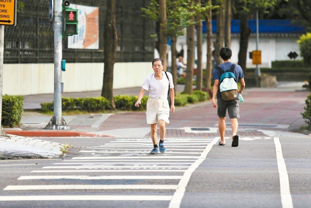
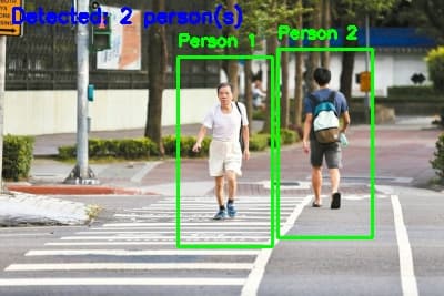
I drew green bounding boxes around the retained regions, added numbered person labels, and displayed a count based on the remaining boxes. I saved that annotated image as result.jpg. The count is therefore the number of retained detections, not an independently verified count of all people in the scene. The script also draws raw candidate rectangles on a separate working copy, but does not save that copy as an additional output.

The report shows two labeled detections, and the completed root script contains the resize, detector, suppression, labeling, count, and save steps. The underlying two-person sample also appears in the reference README; it is one documented example, not evidence of a second independent evaluation. I did not establish dataset-level accuracy or real-time throughput.

The principal learning was how much work sits around a supplied detector. Input scale affects what detail reaches it, overlap suppression determines which boxes remain, and annotation determines whether the output can be checked easily. A broader evaluation would need varied scenes and explicit false-positive and missed-detection records; the existing sample does not establish those behaviors.

These applications came later in the learning sequence. To explain how I reached them, the next sections return to the system-building and interface work that developed my understanding of the Pi as a Linux target.

The foundational work began with the distinction between the build host and the target. I used ARM cross-compilation tools and worked with a sysroot containing target headers and libraries. This helped me understand why a program intended for ARM needs more than a compiler with a different name: its ABI, headers, and linked libraries must also match the target environment.

I practiced remote debugging with QEMU and GDB, separating the environment executing an ARM user program from the debugger controlling it. The workflow introduced the relationship between the executable's debugging information, the remote connection, breakpoints, and inspection of registers and memory. This was a user-program debugging exercise, not evidence of physical JTAG debugging or a complete kernel-debugging session.

Buildroot extended that host–target relationship to a Linux system. I selected a Raspberry Pi configuration and worked through source preparation, menu configuration, and the build process. The recorded filesystem settings include ext4 image generation and a gzip-compressed root-filesystem archive.

The deployment work made the boot components easier to distinguish. Raspberry Pi firmware and boot configuration participate in loading the system; the kernel supplies its core execution environment; device-tree data describes hardware; and the root filesystem provides the files and user-space programs available after startup. I worked with these components and their placement on the SD card. The materials also cover U-Boot as a bootloader option, but I do not treat it as an enabled component of the recorded configuration.

I prepared FAT boot and Linux root partitions, mounted them, and deployed the relevant files or filesystem images. This exposed an important distinction between formatting a partition and writing an image over it: the image's contents determine the resulting filesystem, regardless of an earlier formatting command.

For image inspection, I used partition information to calculate byte offsets from starting sectors and mounted image regions through loop devices. I also practiced whole-card and partition copying with dd, file-level copying with rsync, and serial-console access at 115200 baud.

The records include completed dd copies and a separate image-creation attempt that reported No space left on device, along with a read-only warning during partition inspection. They do not establish a completed recovery from that failure or a restore-and-boot test. Similarly, the Buildroot report preserves configuration screenshots and the boot-check procedure I carried out, but not a captured target boot session. Keeping those distinctions clear helps identify which checks need better records in a reproducible follow-up.

The main lesson was that an embedded environment is a set of connected artifacts. Building a kernel, placing it on storage, selecting the correct root filesystem, and reaching a console are related responsibilities, each requiring its own verification.

Once I had worked through system configuration, I wanted to follow a request from a user program into kernel code. I implemented a small system-call exercise, added the relevant build and dispatch entries, rebuilt and deployed the kernel, and invoked the call from a cross-compiled test program.

The target log contains the custom Hello System Call. message. That gave me an observable result at the boundary I was studying: the user-space invocation reached the kernel implementation. It also made clear that adding a function alone is insufficient; the kernel build and architecture-specific dispatch configuration must connect it to the calling interface.

Kernel modules introduced a different workflow. I compiled a module, transferred its output to the target, used insmod and rmmod, and inspected initialization and exit messages with dmesg. One recorded transfer failed with cp: cannot stat 'hello.ko'. Changing to the directory containing the build output and repeating the copy addressed that specific path error.

The logs also contain earlier Module has invalid ELF structures messages, followed by successful initialization in a later attempt. The records do not establish the exact cause or correction for those ELF failures, so I would not attribute them to a particular architecture or configuration mismatch without further investigation.

A character-device exercise connected a device node to operations initiated from user space. The captured logs show open, ioctl, read, and close callbacks. A separate duplicate-name warning remains in the record; the callback messages demonstrate that those operations were exercised, rather than establishing a fully resolved or production-ready driver.

These implementations taught me to verify integration at the interface being tested. A successful build produces an artifact, while kernel messages and device-operation logs show additional steps in its interaction with the running system.

GPIO work connected the software interfaces to visible physical outputs. I used C and libgpiod with an LED circuit, working through line identification, output configuration, value changes, and resource release.

The TM1637 display added a more structured interaction. Instead of changing one output value, I needed to generate a sequence over CLK and DIO, map decimal digits to segment patterns, select display addresses, and send update and clear commands. The recorded implementation used GPIO25 for CLK and GPIO24 for DIO and included start/stop signaling and countdown logic.

I worked with line acquisition, byte transmission, display functions, and cleanup as separate responsibilities. This made the progression from an LED to a display concrete: controlling a peripheral means coordinating signal transitions and data representation, not simply setting a pin high or low. The TM1637's two-wire protocol also needs to be understood on its own terms rather than assumed to be standard I²C.

The reports preserve completed display routines and wiring photographs. Working through these steps taught me to coordinate signal sequencing, data representation, and resource management in user-space GPIO programming.

I extended the learning journey with TVM experiments involving model compilation, a target runtime, and RPC communication with the Pi. Configuring LLVM support and working with separate build and runtime components introduced another version of the host–target boundary: the machine compiling a model does not have to be the device executing it.

The records include an output vector and terminal outputs associated with several optimization levels. They also contain stalled build attempts and incomplete memory and local-versus-remote comparisons. Without a complete demonstration script and repeatable measurement method, those observations remain exploratory results rather than a performance claim.

I also documented a proposed astronomical observation system connecting camera control, location and sky information, tracking, capture, and a remote interface. It remains a system-design proposal, separate from the implemented experiments.

Across the project, I learned to follow several boundaries: host and target, kernel and user space, software and physical signals, and image input and recognition output. The strongest results were the ones I could inspect directly—kernel messages, device-operation logs, wiring and implementation records, and annotated application outputs.

The next improvement is reproducibility. I would preserve exported build configurations and environment versions, organize application and peripheral source, and pair each implementation with a clear verification record. For the vision work, I would also use a more varied test set and separate preprocessing changes from measured recognition outcomes. That would turn the existing experimental record into a more consistent basis for repeating and extending the work.